Assignment 10 - Parametric Curves
Faith Hoyt
A parametric curve in the plane is a pair of functions x=f(t) and y=g(t) where the two continuous functions define ordered pairs (x,y). The two equations are usually called the parametric equations of a curve. The extent of the curve will depend on the range of t.
We want to investigate what happens to our following functions as we vary a and b with our range being ![]() .
.
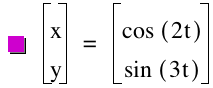
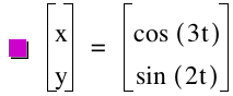
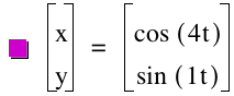
x = cos(at)
y = sin(bt)
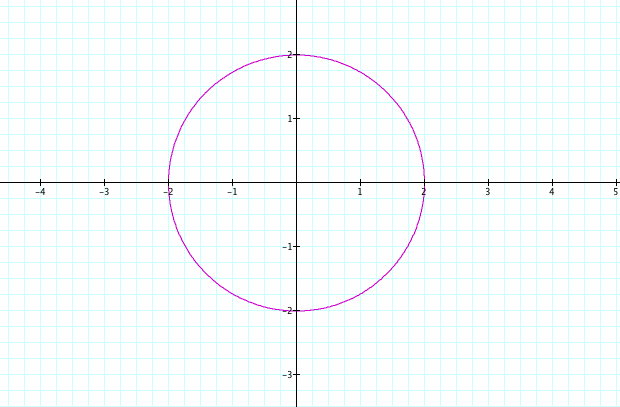
What happens if we let both of our variables equal each other? In this case we will set a = b = 1.
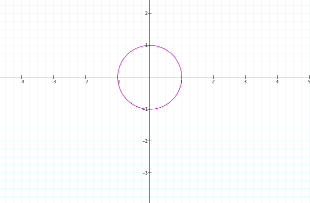
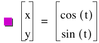
Notice that we get a circle with a radius of 1. If we set our a and b equal to another number, say 3, we still have a circle with a radius of one. Same is true if we set our a and b variables equal to -1.
What happens if a<b?
First, let's see what happens when we let a = 1 and b = 3
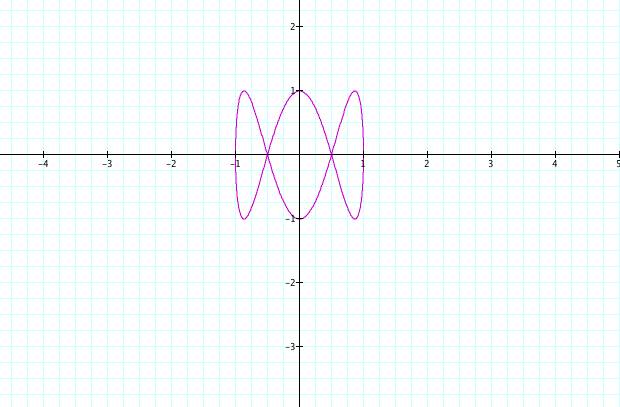
Notice that our graph has what appears to be 3 "loops." The graph is oriented along the x-axis, which corresponds to our cosine function. If we were to took look at just one revolution of the graph, it follows what appears to be the cosine pattern.
In playing with the graph and the variables, I noticed that if I were to multiply both a and b by the same constant, I would get the same graph. One example of this is when I multiplied a and b by 2 to result in a = 2 and b = 6, which gave me the same graph.
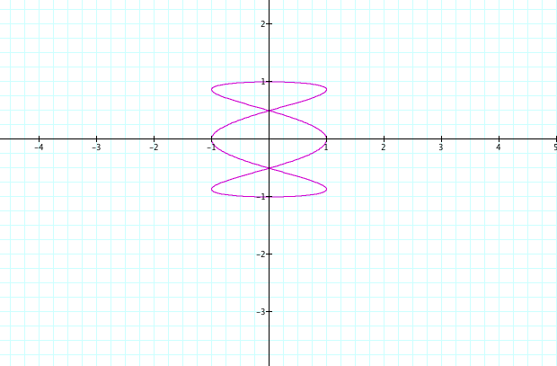
Now, let a = 2 and b = 4.

Once again our graph lies along the x-axis. However, this graph, if we were to look at one revolution, follows the pattern of a sine graph. Again, if I were to multiply my variables by the same constant I would get the same graph. This is true for both positive and negative constants.
Now, let's look at a = 2 and b = 3.
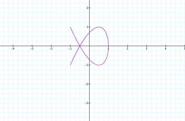
This graph lies along the x-axis. Notice, this graph does not seem to be complete as it has two tails on the left side. It holds true that if we multiply our variables by the same constant then we will get the same graph. It does seem, by looking at the graph, that the there is an invisible box that is formed for x = -1 and 1 and for y = -1 and 1. Do you think this have something to do with our choices for a and b?
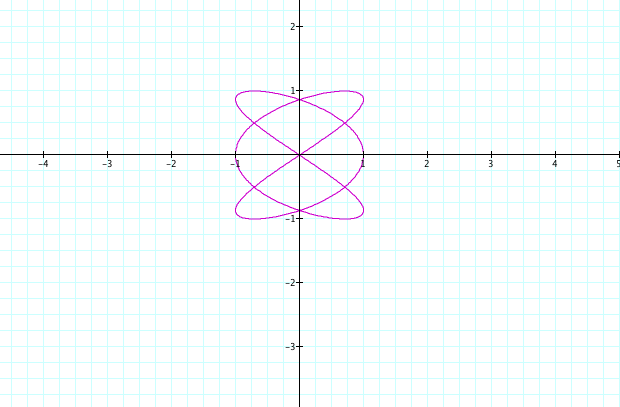
Finally, we will look at our graph when a = 1 and b = 4.
![]()
Notice that this graph is similar to our first graph we looked at. Now, however, it has 4 "loops" rather than 3. Thus, one can conclude that when a =1 the value of b will determine how many "loops" we will get in our graph. Also, we can see that our graph follows the pattern of a sine graph.
What if a > b?
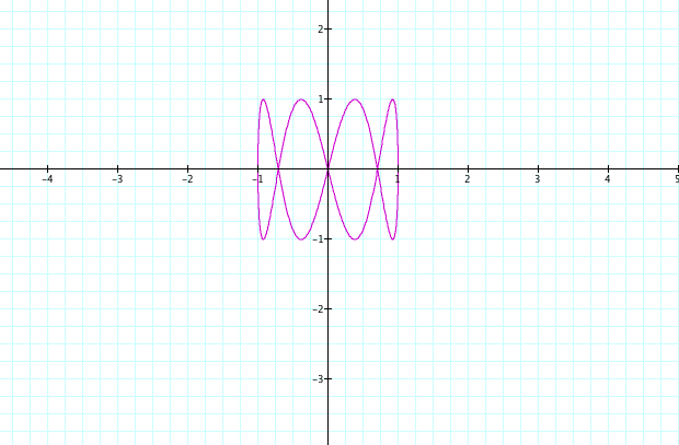
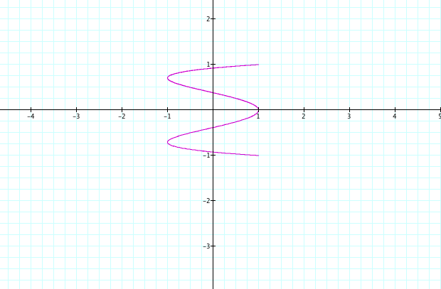
Let's let a = 2 and b = 1
![]()
This graph once again seems to be held in an invisible box. It doesn't even seem like it was able to make one full revolution. One thing to note is that it seems to be oriented around the y-axis. Once again, if we multiply our variables by the same constant, we will get the same graph as a result.
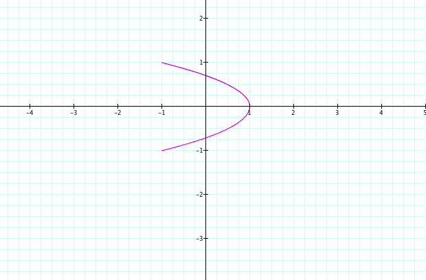
Let's let a = 3 and b = 1.
![]()
This graph is very similar to one we saw above. In fact, it is the same graph as when a = 1 and b = 3, only this time it is oriented around the y-axis. So, we can make the same observations as before. The graph seems to follow the cosine pattern, there are 3 "loops," and if we were to multiply it by the same constant we will get the same graph again.
Let a = 3 and b = 2.
This graph is much different than our other graphs we have seen. Again, it is held inside that invisible box that we have discussed before. There really doesn't seem to be much of a sine or cosine pattern in the graph.
Let a = 4 and b = 1
This graph seems to be a cosine graph on its side that's oriented around the y-axis. Though we looked at the graph for when a and b were switched above, these two graphs are not alike in any way.
From our investigations we can make a few conclusions:
We want to investigate what happens to our following functions as we vary a and b with our range being ![]() .
.
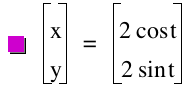
x = a cos(t)
y = b sin(t)
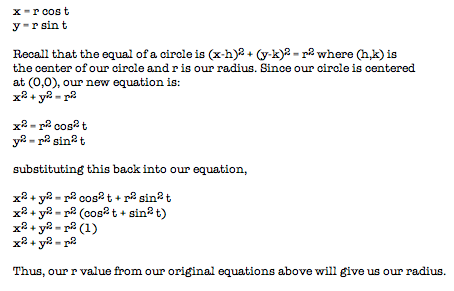
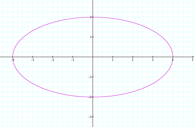
First, let's look at what happens when a = b. In this case we will set both equal to 2.
When our variables are equal, we can use this value to determine the value of the radius of our circle. For example, with our picture above, a = b = 2 and our radius of the circle is 2. Now, we can also prove this:
What if a > b?
When both variables are even, we will get an ellipse. Since our a value is larger than our b value, it is going to have a major axis on the x-axis. Below is an example where a = 4 and b = 2.

Now, if both of our variables are odd, we are going to once again get an ellipse. The major axis is still going to be on the x-axis since our a value is still larger. The affect that a and b have on the graph simply changes the thickness of the ellipse. An example can be seen below where a = 5 and b = 3.
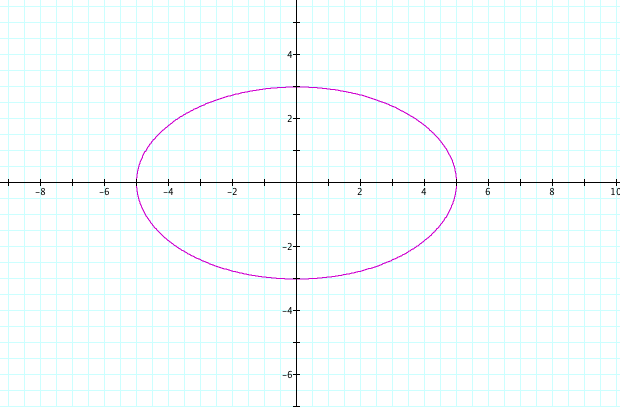
![]()
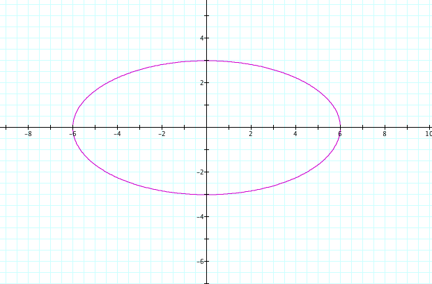
Now, what if there is an even and an odd number for our variables? We will still get an ellipse and our major axis is still going to be on the x-axis. Below is an example where a = 6 and b = 3.

What if a < b?
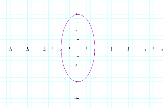
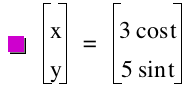
When both of our variables are even we are going to have an ellipse. However, this time our major axis is going to be on the y-axis. This can be seen because our larger variable is with the y equation. Our intersection points on our axis are going to be the same as our a and b values. Below is an example where a = 2 and b = 4.

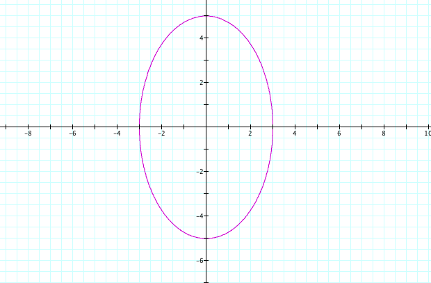
Now, what if both of our variables are odd? We will once again get an ellipse. It will still be oriented about the y-axis. Below we can see an example of what this will look like. Let a = 3 and b = 5. Notice that our ellipse intersects our x-axis at 3 and -3 and that our ellipse intersects our y- axis at 5 and -5.
Finally, let's look at what happens when we have an odd value and an even value. We already know that which variable is larger determines around which axis the ellipse will be oriented. And, once again, a and b determine what the x and y intercepts are. Below is an example of such a graph, where a = 3 and b = 4.
We can see that when we vary our a and b values whether inside our sine or cosine function or outside our functions, it has a great affect on our graphs. When our variables are inside our function it affects the type of graph we get. If our variables are outside our function, they will affect the size of the radius of a circle if they are equal or the semi-major or -minor axis of the ellipse if they are different values. Whichever variable is larger will control the location of the major axis.
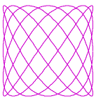
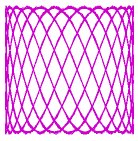
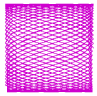
In the case of having our variables inside our function, as they get larger and further apart, the graphs begin to look crazier and crazier. Here are a few pictures of these graphs to show just how complicated it can get.